9장: Tensorflow 시작하기 (p.295)
https://datascienceschool.net/view-notebook/5cbab09d777841f591a67928d7043f51/
Tensorflow를 잘 소개한 링크
소개 :
머신러닝을 다루는 데에 아주 전문적이고 강력한 오픈소스 소프트웨어 라이브러리로 대규모 데이터를 처리하는 데에 아주 좋다. python 위에서 돌아가며 c++ 코드를 사용해 연산을 수행하여 매우 빠르고 효율적으로 실행한다. Tensorflow의 개념은 계산 그래프 computation graph다.

여러 CPU, GPU 등을 사용하여 병렬로 처리할 수 있어 분산 컴퓨팅을 지원한다.
버전 : python 3.6.8버전 ( 3.7이상은 아직 tensorflow 호환이 안되는 줄 앎)
첫 번째 계산 그래프 만들어 세션에서 실행하기
|
1 2 3 4 5 6 7 8 9 10 11 12 13 14 15 16 |
import os os.environ['TF_CPP_MIN_LOG_LEVEL'] = '2' #warning 메시지 안보이기 import matplotlib.pyplot as plt import numpy as np import tensorflow as tf x = tf.Variable(3, name='x') y = tf.Variable(4, name='y') f = x*x*y + y + 2 sess = tf.Session() sess.run(x.initializer) sess.run(y.initializer) result = sess.run(f) print(result) sess.close() |
결과 :![]()
|
1 2 3 4 5 |
with tf.Session() as sess: x.initializer.run() y.initializer.run() result = f.eval() print(result) |
with 블록 안에서는 with 문에서 선언한 세연이 기본 세션으로 지정된다. 코드를 읽고 쓰기가 수월하고 wiht문이 끝나면 세션은 자동으로 종료된다.
|
1 2 3 4 5 6 |
init = tf.global_variables_initializer() with tf.Session() as sess: init.run() result = f.eval() print(result) |
각 변수의 초기화를 일일이 하는 대신 위의 함수를 사용할 수 있다. 이 함수는 초기화를 바로 수행하지 않고 계산 그래프가 실행될 때 모든 변수를 초기화할 노드를 생성한다.
일반적으로 tensorflow는 구성단계, 실행단계 > 두 단계로 구성된다.
계산그래프 관리
노드를 만들면 자동으로 기본 계산 그래프에 추가된다.
|
1 2 |
x1 = tf.Variable(1) print(x1.graph is tf.get_default_graph()) # 기본그래프가 맞냐? |
![]()
가끔 독립적인 계산 그래프를 만들어야 할 때가 있으면 다음과 같이 사용한다.
|
1 2 3 4 5 6 |
graph = tf.Graph() with graph.as_default(): x2 = tf.Variable(2) print(x2.graph is graph)# 새로 생긴 그래프냐? print(x2.graph is tf.get_default_graph()) # default 그래프냐? |
![]()
노드 값의 생애주기
|
1 2 3 4 5 6 7 8 |
w = tf.constant(3) x = w + 2 y = x + 5 z = x * 3 with tf.Session() as sess: print(y.eval()) # 10 print(z.eval()) # 15 |
세션에서 y를 평가하기 위해 그래프를 실행 하는데 y가 x에 의존, x가 w에 의존하는 것을 감지해서 w를 평가하고 x를 평가한 뒤 y를 평가하여 y를 반환한다. 그 다음 z를 평가하는데 전에 쓰인 그래프를 사용하지 않고 x에 의존, x가 w에 의존하는 것을 다시 계산한다. 즉 모든 노드의 값은 계산 그래프 실행 간에 유지되지 않는다.
변수 값은 예외로 그래프 실행 간에도 세션에 의해 유지된다. 변수는 초기화될 때 일생이 시작되고 세션이 종료될 때까지 남아 있는다.
|
1 2 3 4 |
with tf.Session() as sess: y_val, z_val = sess.run([y,z]) print(y_val) print(z_val) |
효율적으로 평가하려면 텐서플로가 한 번의 그래프에서 모두 평가하도록 해야한다.
텐서플로를 이용한 선형 회귀
|
1 2 3 4 5 6 7 8 9 10 11 12 13 14 15 16 17 18 19 20 21 22 23 24 25 26 27 |
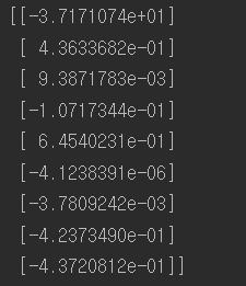
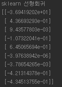
from sklearn.datasets import fetch_california_housing #선형회귀 housing = fetch_california_housing() #캘포 주택가격 데이터셋 m, n = housing.data.shape #데이터셋을 m,n에추출 m(20640,) n( 8 ) #편향에 해당하는 가중치를 같이 계산하기 위해 1값 추가 housing_data_plus_bias = np.c_[np.ones((m,1)), housing.data] X = tf.constant(housing_data_plus_bias, dtype=tf.float32, name="X") # target (20640,1) y = tf.constant(housing.target.reshape(-1,1), dtype=tf.float32, name="y") XT = tf.transpose(X) theta = tf.matmul(tf.matmul(tf.matrix_inverse(tf.matmul( XT ,X )) ,XT) ,y) print(housing.target.shape) with tf.Session() as sess: theta_value = theta.eval() print(theta_value) #사이킷런 모델사용 from sklearn.linear_model import LinearRegression lin_reg = LinearRegression() lin_reg.fit(housing.data, housing.target.reshape(-1, 1)) print("sklearn 선형회귀") print(np.r_[lin_reg.intercept_.reshape(-1, 1), lin_reg.coef_.T]) |
텐서플로를 사용한 것과 사이킷런에서 선형회귀모델을 사용한 코드를 비교한 결과 거즘 똑같은 것을 볼 수 있다. 하지만 연산속도에 차이가 있다.
경사 하강법 구현
직접그래디언트 계산
|
1 2 3 4 5 6 7 8 9 10 11 12 13 14 15 16 17 18 19 20 21 22 23 24 25 26 27 28 29 30 31 32 33 34 35 36 37 38 39 40 41 42 43 44 45 46 47 |
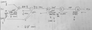
#경사하강법구현 from sklearn.preprocessing import StandardScaler scaler = StandardScaler() #표준화된 데이터를 변환후 저장한다. scaled_housing_data = scaler.fit_transform(housing.data) #스케일된 데이터에 편향가중치벡터를 특성 맨 앞에 추가한다. scaled_housing_data_plus_bias = np.c_[np.ones((m,1)),scaled_housing_data] reset_graph() #graph 초기화 n_epochs = 1000 learning_rate = 0.1 #bias가 추가된 9개의 특성을 가진 데이터를 X에 삽입 X = tf.constant(scaled_housing_data_plus_bias, dtype=tf.float32, name="X") #reshape을 통한 열 생성후 y에 정답 데이터 삽입 y = tf.constant(housing.target.reshape(-1,1), dtype=tf.float32, name="y") #가중치벡터를 -1~ 1사이의 균등분포를 따르는 (9,1) 만큼의 데이터 형성 theta = tf.Variable(tf.random_uniform([n+1,1], -1.0,1.0), name="theta") # X(20640,9) theta(9,1) y_pred = (20640,1) y_pred = tf.matmul(X,theta, name="predictions") error = y_pred - y #(20640,1) # 1/20640 * sumation{(error)^2} mse = tf.reduce_mean(tf.square(error), name="mse") # > 스칼라값 #chain rule에 의해 X의 전치(9,20640)와 error(20640,1) 행렬곱으로 가중치의 미분행렬뽑아낼수 있음. #그림참조 gradients = 2/m * tf.matmul(tf.transpose(X),error) #tf.assign은 변수 저장함수 training_op = tf.assign(theta, theta - learning_rate * gradients) init = tf.global_variables_initializer() with tf.Session() as sess: sess.run(init) #1000번 for epoch in range(n_epochs): if epoch % 100 == 0: print("Epoch", epoch, "MSE = ",mse.eval()) sess.run(training_op) best_theta = theta.eval() print("best_theta :\n",best_theta) |
과정 중 오차역전파를 하기위한 chain rule 계산 그래프:

자동미분사용
위의 코드예시와 같이 gradient를 수학적으로 유도해야 하는데 매우 번거롭고 실수하기 쉽다. symbolic differentiation을 사용해 자동으로 편미분 방정식을 구할 수 있다. 하지만 결과 코드의 효율이 몹시 나쁠 수 있다.
자동으로 gradient를 계산하는 대표적인 4가지 방식

이하 4가지 방식의 이론:

수치미분 구현코드 :
|
1 2 3 4 5 6 7 8 9 10 |
def f(x,y): return x**2*y + y + 2 def deriivate(f, x ,y, x_eps, y_eps): return ((f(x+x_eps, y+ y_eps) - f(x,y) )/ (x_eps + y_eps)) df_dx = deriivate(f,3,4, 0.00001, 0) df_dy = deriivate(f,3,4, 0, 0.00001) print(df_dx) print(df_dy) |
결과 : ![]()

전진모드동작미분은 보는 것과 같이 파라미터 개수만큼 그래프를 계산해야하기 때문에 연산횟수가 많다. 드디어 backprobagation 개념에 왔다. chain rule 성질 덕분에 계산이 매우 용이하다. (텐서플로가 사용하는 방식) 이하 gradient를 오차역전파로 구하는 방법은 다른 게시물 참조.
다양한 자동미분 사용방법
|
1 2 3 4 |
gradients = 2/m * tf.matmul(tf.transpose(X),error) gradients = tf.gradients(mse, [theta])[0] optimizer = tf.train.GradientDescentOptimizer(learning_rate=learning_rate) optimizer = tf.train.MomentumOptimizer(learning_rate=learning_rate, momentum=0.9) |
1. 직접 gradient를 구한 것
2. tf.gradients 함수
3. GradientDescentOptimizer는 경사하강기울기(학습률)까지 갖고있는 모듈
4. 모멘텀 기울기 모듈
데이터주입
tf.placeholder 개념 : 값을 받는 컨테이너박스라 생각하자.
|
1 2 3 4 5 6 7 8 9 |
A = tf.placeholder(tf.float32, shape=(None,3)) B = A + 5 with tf.Session() as sess: B_eval_1 = B.eval(feed_dict= {A : [[1,2,3]]}) B_eval_2 = B.eval(feed_dict= {A : [[4,5,6],[7,8,9]]}) print(B_eval_1) print(B_eval_2) |
텐서플로의 랭크는 배열의 차원을 의미하며 스칼라는 0 벡터는 1 행렬은 2가 된다. linear algebra에서 Rank의 개념과 무관하다.(주의)
tf.placeholder는 Rank가 같아야한다.
tf.placeholder를 이용한 gradient 구현 (mini batch까지)
|
1 2 3 4 5 6 7 8 9 10 11 12 13 14 15 16 17 18 19 20 21 22 23 24 25 26 27 28 29 30 31 32 33 34 35 36 37 38 39 40 41 42 43 44 45 46 47 48 49 50 51 52 53 54 |
#placeholder 구현 n_epochs = 1000 learning_rate = 0.1 # (None,9)형태로 받을수 있는 컨테이너 X = tf.placeholder(tf.float32, shape=(None, n+1), name="X") # (None,1)형태로 받을수 있는 컨테이너 y = tf.placeholder(tf.float32, shape=(None, 1), name="y") #seed=42로 고정 결과값 같게 유지 (9,1) theta = tf.Variable(tf.random_uniform([9,1], -1,1, seed=42), name="theta") # X theta 행렬곱 = (None,1) y_pred = tf.matmul(X,theta, name="predictions") #(None,1) - (None,1) error = y_pred - y mse = tf.reduce_mean(tf.square(error), name="mse") optimizer = tf.train.GradientDescentOptimizer(learning_rate=learning_rate) training_op = optimizer.minimize(mse) init = tf.global_variables_initializer() n_epochs = 10 batch_size = 100 # (20640 / 100) = 206번 = n_batches n_batches = int(np.ceil(m / batch_size)) def fetch_batch(epoch, batch_index, batch_size): #시행마다 다른 결과를 랜덤하게 나타내기위해 seed번호를 다르게줌 np.random.seed(epoch * n_batches + batch_index) #20640개의 데이터중에 100개를 랜덤으로 뽑아서 그 배열을 indices에 저장 indices = np.random.randint(m, size=batch_size) #100개의 배열index만큼 X_batch와 y_batch 추출 X_batch = scaled_housing_data_plus_bias[indices] y_batch = housing.target.reshape(-1,1)[indices] return X_batch, y_batch with tf.Session() as sess: sess.run(init) #n_epochs = 10 206번을 돌면 1epoch 그걸 10번더 for epoch in range(n_epochs): for batch_index in range(n_batches): #206 #fetch_batch매개변수로 epoch,batch_index는 단지 random한 결과를 위해 X_batch, y_batch = fetch_batch(epoch, batch_index, batch_size) sess.run(training_op, feed_dict={X : X_batch, y : y_batch}) best_theta = theta.eval() print(best_theta) |
모델저장과 복원
훈련시킨 모델의 파라미터 , 또는 훈련 중에 epoch마다의 데이터를 저장할 수 있다.
tf.train.Saver() 함수사용
|
1 2 3 4 5 6 7 8 9 10 11 12 13 14 15 16 17 18 19 20 21 22 23 24 25 26 27 28 29 30 31 32 33 34 35 36 37 |
#모델저장 save_file_checkpoint = "C:\\Users\\고영민\\workspace\\parametersave\\my_model.ckpt" save_file_final = "C:\\Users\\고영민\\workspace\\parametersave\\my_model_final.ckpt" reset_graph() n_epochs = 1000 # not shown in the book learning_rate = 0.01 # not shown X = tf.constant(scaled_housing_data_plus_bias, dtype=tf.float32, name="X") # not shown y = tf.constant(housing.target.reshape(-1, 1), dtype=tf.float32, name="y") # not shown theta = tf.Variable(tf.random_uniform([n + 1, 1], -1.0, 1.0, seed=42), name="theta") y_pred = tf.matmul(X, theta, name="predictions") # not shown error = y_pred - y # not shown mse = tf.reduce_mean(tf.square(error), name="mse") # not shown optimizer = tf.train.GradientDescentOptimizer(learning_rate=learning_rate) # not shown training_op = optimizer.minimize(mse) # not shown init = tf.global_variables_initializer() saver = tf.train.Saver({"Weights" : theta}) with tf.Session() as sess: sess.run(init) for epoch in range(n_epochs): if epoch % 100 == 0: print("Epoch", epoch, "MSE =", mse.eval()) # not shown save_path = saver.save(sess, save_file_checkpoint) sess.run(training_op) best_theta = theta.eval() save_path = saver.save(sess, save_file_final) saver.restore(sess, save_file_final) best_theta_restored = theta.eval() print(np.allclose(best_theta,best_theta_restored)) |
![]()
np.allclose 함수는 두 개매변수로 받은 값이 어떤 아주 작은 값보다 작은 차이 값을 가지면 같은 것으로 간주하고 True를 출력하는 함수다.

저장장소를 지정해 그쪽에 파라미터들을 저장할 수 있다.
|
1 2 3 4 5 6 7 8 9 10 11 12 13 14 15 16 17 18 19 20 |
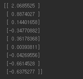
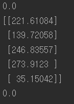
import tensorflow as tf from sklearn.preprocessing import StandardScaler import numpy as np def reset_graph(seed=42): tf.reset_default_graph() tf.set_random_seed(seed) np.random.seed(seed) reset_graph() saver = tf.train.import_meta_graph("C:\\Users\\고영민\\workspace\\parametersave\\my_model_final.ckpt.meta") theta = tf.get_default_graph().get_tensor_by_name("theta:0") with tf.Session() as sess: saver.restore(sess, "C:\\Users\\고영민\\workspace\\parametersave\\my_model_final.ckpt") best_theta_restored = theta.eval() print(best_theta_restored) |
저장한 데이터를 부를 수 있다.
아오 텐서보드는 예전에도 지금도 여전히 안됨 ㅡㅡ(언젠가 하고만다.)
이름 범위
앞으로 쓰게 될 신경망처럼 여러 layer를 가지게 될 경우 복잡하게 되어 헷갈리게 된다. 이를 방지하기 위해 tf.name_scope를 사용할 수 있는데, 말 그대로 이름범위를 만들어 관련 있는 노드들을 그룹으로 묶는 것이다.
|
1 2 3 4 5 |
with tf.name_scope("loss") as scope: error = y_pred - y # not shown mse = tf.reduce_mean(tf.square(error), name="mse") # not shown print(error.op.name) print(mse.op.name) |
![]() loss 라는 이름범위로 묶여있는 것을 볼 수 있다.
loss 라는 이름범위로 묶여있는 것을 볼 수 있다.
모듈화
이름범위로 묶은 것처럼 반복적인 작업은 모듈화로 간단하게 줄일 수 있고 깔끔하게 표현됨으로써 효율을 올릴 수있다.
들어가기전 처음 접한 python 용어:
|
1 2 3 4 5 6 7 8 |
def sum(a): return a + a + a a = 1 result = [sum(a) for i in range(5)] print(result) result = np.reshape(result,(5,1)) print(result) |
result = [function(x) for i in range(y) : 어떤 function(x)를 y번 동안 반복하여 얻어진 결과를 result에 배열로써 저장한다.

비효율적인 코드 :
|
1 2 3 4 5 6 7 8 9 10 11 12 13 14 15 16 17 |
reset_graph() n_features = 3 X = tf.placeholder(tf.float32, shape=(None, n_features), name="X") w1 = tf.Variable(tf.random_normal((n_features, 1)), name="weights1") w2 = tf.Variable(tf.random_normal((n_features, 1)), name="weights2") b1 = tf.Variable(0.0, name="bias1") b2 = tf.Variable(0.0, name="bias2") z1 = tf.add(tf.matmul(X, w1), b1, name="z1") z2 = tf.add(tf.matmul(X, w2), b2, name="z2") relu1 = tf.maximum(z1, 0., name="relu1") #z1, 0중 큰것 출력 relu2 = tf.maximum(z2, 0., name="relu2") # Oops, cut&paste error! Did you spot it? output = tf.add(relu1, relu2, name="output") |
반복되는 구문들이 많다. 이를 다음과 같이 줄일 수 있다.
좀 더 효율적인 코드 :
|
1 2 3 4 5 6 7 8 9 10 11 12 13 14 15 16 |
reset_graph() def relu(X): #X에 데이터가 들어오고 그 데이터형태에서 [1] 즉 특성개수추출 w_shape = (int(X.get_shape()[1]), 1) w = tf.Variable(tf.random_normal(w_shape), name="weights") b = tf.Variable(0.0, name="bias") # 원소별로 더한다. b를 z = tf.add(tf.matmul(X, w), b, name="z") return tf.maximum(z, 0., name="relu") n_features = 3 X = tf.placeholder(tf.float32, shape=(None, n_features), name="X") relus = [relu(X) for i in range(5)] output = tf.add_n(relus, name="output") |
tf.add_n 함수는 텐서의 리스트를 받아 합을 계한하는 연산 노드를 만듭니다.
더 효율적인 모듈화: (name_scope로 범위묶은 것 뿐)
|
1 2 3 4 5 6 7 8 9 10 11 12 13 14 |
def relu(X): with tf.name_scope("relu"): w_shape = (int(X.get_shape()[1]), 1) # not shown in the book w = tf.Variable(tf.random_normal(w_shape), name="weights") # not shown b = tf.Variable(0.0, name="bias") #원소별로 더한다. b를 z = tf.add(tf.matmul(X, w), b, name="z") # not shown return tf.maximum(z, 0., name="max") n_features = 3 X = tf.placeholder(tf.float32, shape=(None, n_features), name="X") relus = [relu(X) for i in range(5)] output = tf.add_n(relus, name="output") |

이처럼 모듈화를 통해 깔끔하게 정리할 수 있다.
변수 공유
반복되는 작업을 통해 변수가 그래프연산마다 동일하게 쓰이지 않고 다르게 인식되어서 메모리가 낭비되는 일이 발생한다. 이를 막는 효율적인 방법이 tf.variable_scope, tf.get_variable 이있다.
|
1 2 3 4 5 6 7 8 9 10 11 12 13 14 15 16 17 18 19 20 21 22 23 24 25 26 27 28 29 30 31 32 33 34 35 36 |
a = np.random.randint(100,size=(5,3)) reset_graph() def relu(X): with tf.variable_scope("relu", reuse=tf.AUTO_REUSE): #변수공유 threshold = tf.get_variable("threshold") w_shape = int(X.get_shape()[1]), 1 # not shown w = tf.Variable(tf.random_normal(w_shape), name="weights") # not shown b = tf.get_variable("b") # not shown z = tf.add(tf.matmul(X, w), b, name="z") # not shown return tf.maximum(z, threshold, name="max") n_features = 3 X = tf.placeholder(tf.float32, shape=(None, n_features), name="X") with tf.variable_scope("relu"): threshold = tf.get_variable("threshold", shape=(), initializer=tf.constant_initializer(0.0)) b = tf.get_variable("b", shape=(), initializer=tf.constant_initializer(0.0)) relus = [relu(X) for relu_index in range(5)] output = tf.add_n(relus, name="output") init = tf.global_variables_initializer() with tf.Session() as sess: sess.run(init) result = sess.run(output, feed_dict={X: a}) print(result) result = sess.run(threshold) print(result) print(tf.global_variables()) |
tf.global_variables()를 해보면 threshold 와 b 는 한 번의 변수로 계속 사용됨을 알 수 있다.
마지막수정 :
|
1 2 3 4 5 6 7 8 9 10 11 12 13 14 15 16 17 18 19 20 21 22 23 24 |
reset_graph() def relu(X): threshold = tf.get_variable("threshold", shape=(), initializer=tf.constant_initializer(0.0)) w_shape = (int(X.get_shape()[1]), 1) # not shown in the book w = tf.Variable(tf.random_normal(w_shape), name="weights") # not shown b = tf.Variable(0.0, name="bias") # not shown z = tf.add(tf.matmul(X, w), b, name="z") # not shown return tf.maximum(z, threshold, name="max") X = tf.placeholder(tf.float32, shape=(None, n_features), name="X") relus = [] for relu_index in range(5): with tf.variable_scope("relu", reuse=(relu_index >= 1)) as scope: relus.append(relu(X)) output = tf.add_n(relus, name="output") init = tf.global_variables_initializer() with tf.Session() as sess: sess.run(init) print(tf.global_variables()) |
References : Hands-On Machine Learning with Scikit Learn & TensorFlow