11장: Deep Neural Network (p.366)
이전포스팅 내용 :
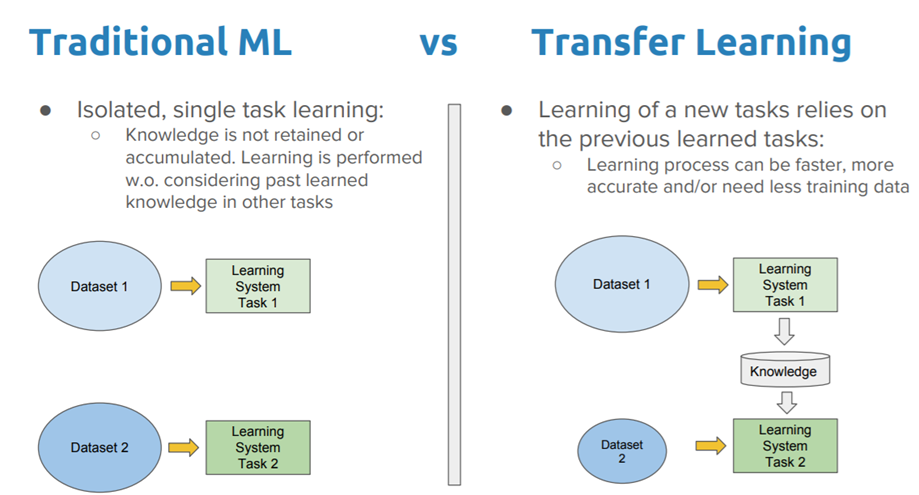
Reusing Pretrained Layers
아주 큰 DNN을 처음부터 학습한다면 좋지 않은 방법이다. 이미 그런 비슷한 부류의 neural network가 존재하는지 보고 존재한다면 하위 층을 가져다 쓸 수 있는 좋은 방법이 있다. (직관적으로도 그러한) 이것을 transfer learning 이라한다. 이 방법은 훈련의 속도를 증가시켜줄 뿐만 아니라 필요한 훈련 데이터도 훨씬적다.
아래 코드는 위의 배치 정규화 코드를 재사용해서 구현한 코드이다.
|
1 2 3 4 5 6 7 8 9 10 11 12 13 14 15 16 17 18 19 20 21 22 23 24 25 26 27 28 29 30 31 32 33 34 35 36 37 38 39 40 41 42 43 44 45 46 47 48 49 50 51 52 53 54 55 56 57 58 59 60 61 62 63 64 65 66 67 68 69 70 71 |
import numpy as np import tensorflow as tf import mnist def reset_graph(seed=42): tf.reset_default_graph() tf.set_random_seed(seed) np.random.seed(seed) reset_graph() saver = tf.train.import_meta_graph("C:\\Users\\고영민\\workspace\\parametersave\\my_batch.ckpt.meta") (X_train, y_train), (X_test, y_test) = mnist.load_mnist(normalize=True) y_train = y_train.astype(np.int32) y_test = y_test.astype(np.int32) X_valid, X_train = X_train[:5000], X_train[5000:] y_valid, y_train = y_train[:5000], y_train[5000:] #------------------------------------------------ #층깊이 n_inputs = 28 * 28 n_hidden1 = 300 n_hidden2 = 100 n_outputs = 10 for op in tf.get_default_graph().get_operations(): print(op.name) X = tf.get_default_graph().get_tensor_by_name("X:0") y = tf.get_default_graph().get_tensor_by_name("y:0") accuracy = tf.get_default_graph().get_tensor_by_name("eval/accuracy:0") training_op = tf.get_default_graph().get_operation_by_name("train/training_op") #또 다른 방법인 collection 추가하기 for op in (X,y,accuracy,training_op): tf.add_to_collection("my_important_ops",op) X,y,accuracy,training_op = tf.get_collection("my_important_ops") def shuffle_batch(X, y, batch_size): rnd_idx = np.random.permutation(len(X)) #예를들어 55000개 n_batches = len(X) // batch_size #len(X)는 X의 행데이터 1100 for batch_idx in np.array_split(rnd_idx, n_batches): X_batch, y_batch = X[batch_idx], y[batch_idx] yield X_batch, y_batch n_epochs = 20 batch_size = 200 with tf.Session() as sess: saver.restore(sess,"C:\\Users\\고영민\\workspace\\parametersave\\my_batch.ckpt") for epoch in range(n_epochs): for X_batch, y_batch in shuffle_batch(X_train,y_train,batch_size): sess.run(training_op,feed_dict={X:X_batch, y:y_batch}) accuracy_val = accuracy.eval(feed_dict={X:X_valid, y:y_valid}) print(epoch, "Validation accuracy:", accuracy_val) |
코드를 보면서 name 의 활용중요성을 느낀다.
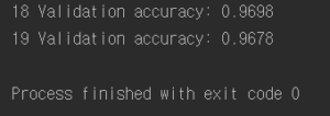
결과 : 
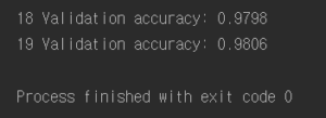
결과를 보면 알다시피 앞선 배치 정규화 때 구해놓은 변수들과 연산자들을 사용하기 때문에 시작부터 높은 정확도를 보이는 것을 볼 수 있다.
하지만 일반적으로 transfer learning을 하려하면 원래 모델의 일부만을(낮은 층) 사용하는 것이기 때문에 다른 방법이 필요하다.
만약 pretrained model의 name이 문서화되어 있지 않으면 그 그래프를 뒤져서 name을 찾아가서 해야할 것이다. 여기서 get_operations() 메서드를 사용할 수 있다. name들이 출력된다. 내가 이 모델을 만든 사람이라면 이 name들을 다른 사람들이 알아보기 쉽게 명료하게 만들어야할 것이다. 또 다른 접근 방법은 사람들이 중요하게 생각하는 연산들을 collection으로 묶는 것이다.
tf.add_to_collection(name,value) 함수:
name : collection의 key 예를 들어, GraphKeys class 에는 collection에 대한 많은 표준 이름이 포함되어 있다.(“my_important_ops”)
value : value를 collection에 추가한다.
이렇게 구현한 collection은 밑에와 같이 간편하게 불려질 수 있다.
|
1 |
X,y,accuracy,training_op = tf.get_collection("my_important_ops") |
tf.get_collection(key, scope=None) 함수:
key : collection의 key 예를 들어, GraphKeys class 에는 collection에 대한 많은 표준 이름이 포함되어 있다.
scope : (optional)
https://eyeofneedle.tistory.com/24 위 함수에 대한 설명이 잘되있음.
일반적인 transfer learning
일반적인 transfer learning을 생각해보자. 먼저 우리는 5개의 hidden layer가 이미 만들어져 훈련되어 있다고 생각해보자. (밑에 코드 처럼)
|
1 2 3 4 5 6 7 8 9 10 11 12 13 14 15 16 17 18 19 20 21 22 23 24 25 26 27 28 29 30 31 32 33 34 35 36 37 38 39 40 41 42 43 44 45 46 47 48 49 50 51 52 53 54 55 56 57 58 59 60 61 62 63 64 65 66 |
#------------------------------------------------------------------새로운모델생성 reset_graph() n_inputs = 28 * 28 # MNIST n_hidden1 = 300 n_hidden2 = 50 n_hidden3 = 50 n_hidden4 = 50 n_hidden5 = 50 n_outputs = 10 X = tf.placeholder(tf.float32, shape=(None, n_inputs), name="X") y = tf.placeholder(tf.int32, shape=(None), name="y") with tf.name_scope("dnn"): hidden1 = tf.layers.dense(X, n_hidden1, activation=tf.nn.relu, name="hidden1") hidden2 = tf.layers.dense(hidden1, n_hidden2, activation=tf.nn.relu, name="hidden2") hidden3 = tf.layers.dense(hidden2, n_hidden3, activation=tf.nn.relu, name="hidden3") hidden4 = tf.layers.dense(hidden3, n_hidden4, activation=tf.nn.relu, name="hidden4") hidden5 = tf.layers.dense(hidden4, n_hidden5, activation=tf.nn.relu, name="hidden5") logits = tf.layers.dense(hidden5, n_outputs, name="outputs") with tf.name_scope("loss"): xentropy = tf.nn.sparse_softmax_cross_entropy_with_logits(labels=y, logits=logits) loss = tf.reduce_mean(xentropy, name="loss") with tf.name_scope("eval"): correct = tf.nn.in_top_k(logits, y, 1) accuracy = tf.reduce_mean(tf.cast(correct, tf.float32), name="accuracy") learning_rate = 0.01 threshold = 1.0 optimizer = tf.train.GradientDescentOptimizer(learning_rate) grads_and_vars = optimizer.compute_gradients(loss) capped_gvs = [(tf.clip_by_value(grad, -threshold, threshold), var) for grad, var in grads_and_vars] training_op = optimizer.apply_gradients(capped_gvs) saver = tf.train.Saver() def shuffle_batch(X, y, batch_size): rnd_idx = np.random.permutation(len(X)) #예를들어 55000개 n_batches = len(X) // batch_size #len(X)는 X의 행데이터 1100 for batch_idx in np.array_split(rnd_idx, n_batches): X_batch, y_batch = X[batch_idx], y[batch_idx] yield X_batch, y_batch init = tf.global_variables_initializer() saver = tf.train.Saver() n_epochs = 20 batch_size = 200 with tf.Session() as sess: sess.run(init) for epoch in range(n_epochs): for X_batch, y_batch in shuffle_batch(X_train, y_train, batch_size): sess.run(training_op, feed_dict={X: X_batch, y: y_batch}) accuracy_val = accuracy.eval(feed_dict={X: X_valid, y: y_valid}) print(epoch, "Validation accuracy:", accuracy_val) save_path = saver.save(sess, "C:\\Users\\고영민\\workspace\\parametersave\\my_new_batch.ckpt") |
그다음 나는 4개의 hiddenlayer를 가진 DNN을 구축할건데 1~3층까지의 hidden layer를 위의 1~3층까지의 훈련된 hiddenlayer를 가져다 쓰고 나머지 4번째 층만 새로 학습시키려한다. 그 코드는 아래와 같다.
|
1 2 3 4 5 6 7 8 9 10 11 12 13 14 15 16 17 18 19 20 21 22 23 24 25 26 27 28 29 30 31 32 33 34 35 36 37 38 39 40 41 42 43 44 45 46 47 48 49 50 51 52 53 54 55 56 57 58 59 60 61 62 63 64 65 66 67 68 |
#hidden layer가 4개인 모델을 만들건데 위에 만들어진 모델의 hidden layer 3층까지를 가져와쓰고 #마지가 4층을 새롭게 훈련하는 코드 reset_graph() n_inputs = 28 * 28 # MNIST n_hidden1 = 300 # reused n_hidden2 = 50 # reused n_hidden3 = 50 # reused n_hidden4 = 20 # new! n_outputs = 10 # new! X = tf.placeholder(tf.float32, shape=(None, n_inputs), name="X") y = tf.placeholder(tf.int32, shape=(None), name="y") with tf.name_scope("dnn"): hidden1 = tf.layers.dense(X, n_hidden1, activation=tf.nn.relu, name="hidden1") # reused hidden2 = tf.layers.dense(hidden1, n_hidden2, activation=tf.nn.relu, name="hidden2") # reused hidden3 = tf.layers.dense(hidden2, n_hidden3, activation=tf.nn.relu, name="hidden3") # reused hidden4 = tf.layers.dense(hidden3, n_hidden4, activation=tf.nn.relu, name="hidden4") # new! logits = tf.layers.dense(hidden4, n_outputs, name="outputs") # new! with tf.name_scope("loss"): xentropy = tf.nn.sparse_softmax_cross_entropy_with_logits(labels=y, logits=logits) loss = tf.reduce_mean(xentropy, name="loss") with tf.name_scope("eval"): correct = tf.nn.in_top_k(logits, y, 1) accuracy = tf.reduce_mean(tf.cast(correct, tf.float32), name="accuracy") learning_rate= 0.01 with tf.name_scope("train"): optimizer = tf.train.GradientDescentOptimizer(learning_rate) training_op = optimizer.minimize(loss) reuse_vars = tf.get_collection(tf.GraphKeys.GLOBAL_VARIABLES, scope="hidden[123]") # regular expression restore_saver = tf.train.Saver(reuse_vars) # to restore layers 1-3 init = tf.global_variables_initializer() saver = tf.train.Saver() def shuffle_batch(X, y, batch_size): rnd_idx = np.random.permutation(len(X)) #예를들어 55000개 n_batches = len(X) // batch_size #len(X)는 X의 행데이터 1100 for batch_idx in np.array_split(rnd_idx, n_batches): X_batch, y_batch = X[batch_idx], y[batch_idx] yield X_batch, y_batch n_epochs = 20 batch_size = 200 with tf.Session() as sess: init.run() restore_saver.restore(sess,"C:\\Users\\고영민\\workspace\\parametersave\\my_new_batch.ckpt") for epoch in range(n_epochs): # not shown in the book for X_batch, y_batch in shuffle_batch(X_train, y_train, batch_size): # not shown sess.run(training_op, feed_dict={X: X_batch, y: y_batch}) # not shown accuracy_val = accuracy.eval(feed_dict={X: X_valid, y: y_valid}) # not shown print(epoch, "Validation accuracy:", accuracy_val) # not shown save_path = saver.save(sess, "C:\\Users\\고영민\\workspace\\parametersave\\my_new_batch_final.ckpt") |
결과: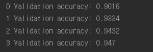

hidden layer 3층까지 훈련된 가중치들을 가져와서 새로운 모델에 적용함으로써 초기부터 높은 정확도를 보이고 보다 적은 데이터를 가지고도 이런 효과를 볼 수 있다는 장점이 있다. 모델이 더욱 더 비슷하다면 더 많은 hidden layer의 훈련된 가중치들을 쓸 수 있다.
Reusing Models from Other Frameworks
다른 frame work의 모델을 재사용하는 것으로 예를 들어 다음은 다른 프레임 워크를 사용해 만든 모델의 첫 번째 은닉층으로부터 가중치와 편향을 어떻게 복사하는지 보여준다.
|
1 2 3 4 5 6 7 8 9 10 11 12 13 14 15 16 17 18 19 20 21 22 23 24 25 26 27 28 29 30 31 32 |
#reusing models from other framework #훈련된 다른 framework로 부터 첫 번째 hidden layer가중치를 어떻게복사하는지 reset_graph() n_inputs = 2 n_hidden1 = 3 original_w = [[1., 2., 3.], [4., 5., 6.]] # Load the weights from the other framework original_b = [7., 8., 9.] # Load the biases from the other framework X = tf.placeholder(tf.float32, shape=(None, n_inputs), name="X") hidden1 = tf.layers.dense(X, n_hidden1, activation=tf.nn.relu, name="hidden1") # [...] Build the rest of the model # Get a handle on the assignment nodes for the hidden1 variables graph = tf.get_default_graph() #/Assign 모든 텐서플로변수는 초기화와 연관된 할당연산을 가지고 있다. # 그 할당연산의 핸들을 가져오는 작업 assign_kernel = graph.get_operation_by_name("hidden1/kernel/Assign") assign_bias = graph.get_operation_by_name("hidden1/bias/Assign") #/Assign으로 할당받을 작업을 마치고 입력받도록 조정하는데 [0]번째는 # 그 변수 자체고 두 번째 입력은 이 변수에 할당될 값이다. init_kernel = assign_kernel.inputs[1] init_bias = assign_bias.inputs[1] init = tf.global_variables_initializer() with tf.Session() as sess: #모든 변수를 초기화할때 위에 있는 변수를 받을 작업을 feed_dict로 함. sess.run(init, feed_dict={init_kernel: original_w, init_bias: original_b}) # [...] Train the model on your new task print(hidden1.eval(feed_dict={X: [[10.0, 11.0]]})) # not shown in the book |
![]()
Freezing the Lower Layers
가중치들이 훈련된 것들을 가져와 사용하는 것은 효율적이다. DNN의 하위층은 이미지에 있는 저수준 특성을 감지하도록 학습되어서 다른 이미지 분류 작업에 유용할 것같다. 즉 이 하위층들은 훈련을 하지 않아도 될 것 같다. 그럼 하위층을 얼리는 것처럼 학습을 못하게 제외시키는 방법이 있다. 아래의 코드를 보면 1,2층의 가중치들을 얼리고 그 상태에서 상위 층을 학습시키는 코드이다. 이런 경우 하위 층이 고정되기 때문에 상위 층의 학습이 더 수월해진다.
|
1 2 3 4 5 6 7 8 9 10 11 12 13 14 15 16 17 18 19 20 21 22 23 24 25 26 27 28 29 30 31 32 33 34 35 36 37 38 39 40 41 42 43 44 45 46 47 48 49 50 51 52 53 54 55 56 57 58 59 |
reset_graph() n_inputs = 28 * 28 # MNIST n_hidden1 = 300 # reused n_hidden2 = 50 # reused n_hidden3 = 50 # reused n_hidden4 = 20 # new! n_outputs = 10 # new! X = tf.placeholder(tf.float32, shape=(None, n_inputs), name="X") y = tf.placeholder(tf.int32, shape=(None), name="y") with tf.name_scope("dnn"): hidden1 = tf.layers.dense(X, n_hidden1, activation=tf.nn.relu, name="hidden1") # reused hidden2 = tf.layers.dense(hidden1, n_hidden2, activation=tf.nn.relu, name="hidden2") # reused hidden3 = tf.layers.dense(hidden2, n_hidden3, activation=tf.nn.relu, name="hidden3") # reused hidden4 = tf.layers.dense(hidden3, n_hidden4, activation=tf.nn.relu, name="hidden4") # new! logits = tf.layers.dense(hidden4, n_outputs, name="outputs") # new! with tf.name_scope("loss"): xentropy = tf.nn.sparse_softmax_cross_entropy_with_logits(labels=y, logits=logits) loss = tf.reduce_mean(xentropy, name="loss") with tf.name_scope("eval"): correct = tf.nn.in_top_k(logits, y, 1) accuracy = tf.reduce_mean(tf.cast(correct, tf.float32), name="accuracy") learning_rate = 0.01 with tf.name_scope("train"): # not shown in the book optimizer = tf.train.GradientDescentOptimizer(learning_rate) #hidden[34]와 출력층에 있는 학습할 변수목록들 train_vars = tf.get_collection(tf.GraphKeys.TRAINABLE_VARIABLES, scope="hidden[34]|outputs") #위의 것들만 학습 training_op = optimizer.minimize(loss, var_list=train_vars) #재사용할 층의 가중치들은 hidden[123] reuse_vars = tf.get_collection(tf.GraphKeys.GLOBAL_VARIABLES, scope="hidden[123]") # regular expression restore_saver = tf.train.Saver(reuse_vars) # to restore layers 1-3 init = tf.global_variables_initializer() saver = tf.train.Saver() n_epochs = 20 batch_size = 200 with tf.Session() as sess: init.run() restore_saver.restore(sess, "C:\\Users\\고영민\\workspace\\parametersave\\my_new_batch_final.ckpt") for epoch in range(n_epochs): for X_batch, y_batch in shuffle_batch(X_train, y_train, batch_size): sess.run(training_op, feed_dict={X: X_batch, y: y_batch}) accuracy_val = accuracy.eval(feed_dict={X: X_valid, y: y_valid}) print(epoch, "Validation accuracy:", accuracy_val) save_path = saver.save(sess, "C:\\Users\\고영민\\workspace\\parametersave\\my_new_batch_final2.ckpt") |
결과 : 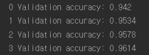
또 다른 방법으로는 stop_gradient() 함수를 layer graph에 추가하는 것이다.
|
1 2 3 4 5 6 7 8 9 10 11 |
with tf.name_scope("dnn"): hidden1 = tf.layers.dense(X, n_hidden1, activation=tf.nn.relu, name="hidden1") # reused frozen hidden2 = tf.layers.dense(hidden1, n_hidden2, activation=tf.nn.relu, name="hidden2") # reused frozen hidden2_stop = tf.stop_gradient(hidden2) hidden3 = tf.layers.dense(hidden2_stop, n_hidden3, activation=tf.nn.relu, name="hidden3") # reused, not frozen hidden4 = tf.layers.dense(hidden3, n_hidden4, activation=tf.nn.relu, name="hidden4") # new! logits = tf.layers.dense(hidden4, n_outputs, name="outputs") # new! |
tf.stop_gradient(input, name=None) 함수:
input을 입력으로 받아 연산 후 출력하는 함수로, gradient를 구할 때 그 연산 그래프에서 제외된다. 즉 학습을 하지 않는다.
즉 위의 코드를 보고 설명하자면 (나머지 코드는 위의 Freezing the Lower layers 코드와 같음) hidden1,2를 stop_gradient로 학습을 제외시킨 뒤, 재사용하는 변수들은 1,2,3층을 사용하여 구현한 것이다.
Caching the Frozen Layers
https://aws.amazon.com/ko/caching/ cache란 무엇인가? 설명
요점은 Frozen layer는 고정되어 있기 때문에 반복적인 학습 연산에서 제외시키고, (메모리가 충분하다면) 전체 훈련데이터셋에 대해 1번만 Frozen layer에 대한 훈련된 가중치들을 대입해 학습시킨다. 그럼 이후부터는 Frozen layer에 대한 불필요한 연산을 막기 때문에 엄청난 속도를 볼 수 있다.
|
1 2 3 4 5 6 7 8 9 10 11 12 13 14 15 16 17 18 19 20 21 22 23 24 25 26 27 28 29 30 31 32 33 34 35 36 37 38 39 40 41 42 43 44 45 46 47 48 49 50 51 52 53 54 55 56 57 58 59 60 61 62 63 64 65 66 67 68 69 70 71 72 73 74 75 76 77 78 79 80 |
#caching reset_graph() n_inputs = 28 * 28 # MNIST n_hidden1 = 300 # reused n_hidden2 = 50 # reused n_hidden3 = 50 # reused n_hidden4 = 20 # new! n_outputs = 10 # new! X = tf.placeholder(tf.float32, shape=(None, n_inputs), name="X") y = tf.placeholder(tf.int32, shape=(None), name="y") with tf.name_scope("dnn"): hidden1 = tf.layers.dense(X, n_hidden1, activation=tf.nn.relu, name="hidden1") # reused frozen hidden2 = tf.layers.dense(hidden1, n_hidden2, activation=tf.nn.relu, name="hidden2") # reused frozen & cached hidden2_stop = tf.stop_gradient(hidden2) hidden3 = tf.layers.dense(hidden2_stop, n_hidden3, activation=tf.nn.relu, name="hidden3") # reused, not frozen hidden4 = tf.layers.dense(hidden3, n_hidden4, activation=tf.nn.relu, name="hidden4") # new! logits = tf.layers.dense(hidden4, n_outputs, name="outputs") # new! with tf.name_scope("loss"): xentropy = tf.nn.sparse_softmax_cross_entropy_with_logits(labels=y, logits=logits) loss = tf.reduce_mean(xentropy, name="loss") with tf.name_scope("eval"): correct = tf.nn.in_top_k(logits, y, 1) accuracy = tf.reduce_mean(tf.cast(correct, tf.float32), name="accuracy") learning_rate = 0.01 with tf.name_scope("train"): optimizer = tf.train.GradientDescentOptimizer(learning_rate) training_op = optimizer.minimize(loss) reuse_vars = tf.get_collection(tf.GraphKeys.GLOBAL_VARIABLES, scope="hidden[123]") # regular expression restore_saver = tf.train.Saver(reuse_vars) # to restore layers 1-3 init = tf.global_variables_initializer() saver = tf.train.Saver() n_epochs = 20 batch_size = 200 n_batches = len(X_train) // batch_size with tf.Session() as sess: start = time.time() init.run() restore_saver.restore(sess,"C:\\Users\\고영민\\workspace\\parametersave\\my_new_batch_final.ckpt") #Freezing을 2층까지 할 것이기 때문에 hidden2 까지를 이미 훈련된 hidden1,2가중치들을 가져와 #한번 돌려서 학습시킨다. 이후에 돌리는 것은 무의미 하기 때문에. h2_cache = sess.run(hidden2, feed_dict={X: X_train}) h2_cache_valid = sess.run(hidden2, feed_dict={X: X_valid}) # not shown in the book for epoch in range(n_epochs): shuffled_idx = np.random.permutation(len(X_train)) hidden2_batches = np.array_split(h2_cache[shuffled_idx], n_batches) y_batches = np.array_split(y_train[shuffled_idx], n_batches) for hidden2_batch, y_batch in zip(hidden2_batches, y_batches): sess.run(training_op, feed_dict={hidden2: hidden2_batch, y: y_batch}) accuracy_val = accuracy.eval(feed_dict={hidden2: h2_cache_valid, # not shown y: y_valid}) # not shown print(epoch, "Validation accuracy:", accuracy_val) # not shown end = time.time() total = end - start print("총 걸린시간 : ",round(total,2), "초") save_path = saver.save(sess, "C:\\Users\\고영민\\workspace\\parametersave\\my_new_batch_final2.ckpt") |
결과 :![]() 총 걸린 시간이 12초 밖에 걸리지 않았다.
총 걸린 시간이 12초 밖에 걸리지 않았다.
References: Hands – On Machine Learning with Scikit-Learn & TensorFlow