4장: 모델 훈련 part 6 (p.188)
Logistic Regression
선형 회귀를 연속적인 것에서 이산적인 것으로 변환하여 분류기처럼 행동하게끔 할수 있게 해주는 방법이다. 주어진 데이터들이 이산적이거나 (성별 0 또는 1) , 연속적인 (키 : 171.2, 173.5cm 등) 변수들을 갖고 있는데 연속적인 데이터 성질 때문에 나오는 출력 값은 연속적이게 된다. 이 연속적인 값을 어떠한 function에서 작업을 통해 0 또는 1 처럼 분류하는 값으로 이끌어낼 수 있다.
확률 추정 / 훈련과 비용함수


굳이 sigmoid 변환을 통해 0과 1 사이의 값으로 즉, 확률적인 성질을 띄게한 이유가 애매하다. 왜냐면 굳이 0 과 1 사이가 아니어도 특정 기준을 잡아 분류기준을 정할 수 있기 때문이다. 하지만 사용한 이유를 보자면 binomial distribution처럼 행동하여 비용함수의 정의를 표현할 때 사용하기 위하여 0과1로 제한한 확률적인 성질로는 적합해보인다. (하지만 이 또한 비용함수를 다른 것으로 정의하면 필요가 없어진다.) 이건 다른 관점의 얘기인데 굳이 시그모이드를 사용한 이유가 궁금해지는데, non-linear한 성질과 monotone increasing function의 성질로 신경망을 학습시킬 때 좋은 효과를 보인다. 시그모이드 말고 ReLu 등의 함수들
사용 예시 ( iris dataset )
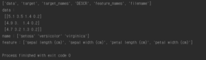
logistic regression을 이용하기 위해 iris dataset을 사용해본다. setosa, versicolor, virginica 세 개의 품종이 있으며 150개의 꽃잎, 꽃받침, 너비, 길이를 가지고 있다.
|
1 2 3 4 5 6 7 8 9 |
#4.6 Logistic Regression iris = datasets.load_iris() print(list(iris.keys())) X = iris["data"][:, 3:] #꽃잎의 너비 y = (iris["target"] == 2).astype(np.int) #버지니아면 1 아니면 0 print("data :",iris.data[:3]) print("name :",iris.target_names[:3]) print("feature :",iris.feature_names) |
logistic regression 을 이용한 훈련코드
|
1 2 3 4 5 6 7 8 9 10 11 12 13 14 15 16 17 18 19 20 21 22 23 24 25 |
log_reg = LogisticRegression() log_reg.fit(X,y) X_new = np.linspace(0,3,1000).reshape(-1,1) y_proba = log_reg.predict_proba(X_new) X_new = np.linspace(0, 3, 1000).reshape(-1, 1) y_proba = log_reg.predict_proba(X_new) decision_boundary = X_new[y_proba[:, 1] >= 0.5][0] plt.figure(figsize=(8, 3)) plt.plot(X[y==0], y[y==0], "bs") plt.plot(X[y==1], y[y==1], "g^") plt.plot([decision_boundary, decision_boundary], [-1, 2], "k:", linewidth=2) plt.plot(X_new, y_proba[:, 1], "g-", linewidth=2, label="Iris-Virginica") plt.plot(X_new, y_proba[:, 0], "b--", linewidth=2, label="Not Iris-Virginica") plt.text(decision_boundary+0.02, 0.15, "Decision boundary", fontsize=14, color="k", ha="center") plt.arrow(decision_boundary, 0.08, -0.3, 0, head_width=0.05, head_length=0.1, fc='b', ec='b') plt.arrow(decision_boundary, 0.92, 0.3, 0, head_width=0.05, head_length=0.1, fc='g', ec='g') plt.xlabel("Petal width (cm)", fontsize=14) plt.ylabel("Probability", fontsize=14) plt.legend(loc="center left", fontsize=14) plt.axis([0, 3, -0.02, 1.02]) plt.show() |

1.6cm 근방에서 decision boundary가 만들어진다. 즉 너비가 1.6cm 보다 크면 분류기는 verginica로 분류하고 그보다 작으면 아니라고 예측할 것이다.
|
1 |
print("1.7cm : ",log_reg.predict([[1.7]]),"\n1.5cm : ",log_reg.predict([[1.5]])) |

이번에는 꽃잎 너비와 길이 두개의 특성으로 보여준다. 점선은 이 모델의 decision boundary이며 이 경계는 선형이다.

Softmax Regression


소프트맥스 회귀를 사용해 붓꽃을 세 개의 클래스로 분류한다. Logistic Regression은 클래스가 둘 이상일 때 기본적으로 OvA 전략을 사용한다. 하지만 multi-class 매개변수를 “multinomial”로 바꾸면 소프트맥스 회귀를 사용할 수 있다. 소프트맥스 회귀를 사용하려면 solver 매개변수에 “lbfgs”와 같이 소프트맥스 회귀를 지원하는 알고리즘을 지정해야 한다.
|
1 2 3 4 5 6 7 8 |
X = iris["data"][:, (2,3)] y = iris["target"] softmax_reg = LogisticRegression(multi_class="multinomial",solver="lbfgs", C=10, random_state=42) softmax_reg.fit(X, y) print(softmax_reg.predict([[5,2]])) print(softmax_reg.predict_proba([[5,2]])) |
![]()
길이가 5, 너비가 2 cm인 붓꽃을 예측해보라고 하면 94.2% 확률로 virginica라고 출력한다.

4장 전체 코드 :
|
1 2 3 4 5 6 7 8 9 10 11 12 13 14 15 16 17 18 19 20 21 22 23 24 25 26 27 28 29 30 31 32 33 34 35 36 37 38 39 40 41 42 43 44 45 46 47 48 49 50 51 52 53 54 55 56 57 58 59 60 61 62 63 64 65 66 67 68 69 70 71 72 73 74 75 76 77 78 79 80 81 82 83 84 85 86 87 88 89 90 91 92 93 94 95 96 97 98 99 100 101 102 103 104 105 106 107 108 109 110 111 112 113 114 115 116 117 118 119 120 121 122 123 124 125 126 127 128 129 130 131 132 133 134 135 136 137 138 139 140 141 142 143 144 145 146 147 148 149 150 151 152 153 154 155 156 157 158 159 160 161 162 163 164 165 166 167 168 169 170 171 172 173 174 175 176 177 178 179 180 181 182 183 184 185 186 187 188 189 190 191 192 193 194 195 196 197 198 199 200 201 202 203 204 205 206 207 208 209 210 211 212 213 214 215 216 217 218 219 220 221 222 223 224 225 226 227 228 229 230 231 232 233 234 235 236 237 238 239 240 241 242 243 244 245 246 247 248 249 250 251 252 253 254 255 256 257 258 259 260 261 262 263 264 265 266 267 268 269 270 271 272 273 274 275 276 277 278 279 280 281 282 283 284 285 286 287 288 289 290 291 292 293 294 295 296 297 298 299 300 301 302 303 304 305 306 307 308 309 310 311 312 313 314 315 316 317 318 319 320 321 322 323 324 325 326 327 328 329 330 331 332 333 334 335 336 337 338 339 340 341 342 343 344 345 346 347 348 349 350 351 352 353 354 355 356 357 358 359 360 361 362 363 364 365 366 367 368 369 370 371 372 373 374 375 376 377 378 379 380 381 382 383 384 385 386 387 388 389 390 391 392 393 394 395 396 397 398 399 400 401 402 403 404 405 406 407 408 409 410 411 412 413 414 415 416 417 418 419 420 421 422 423 424 425 426 427 428 429 430 431 432 433 434 435 436 437 438 439 440 441 442 443 444 445 446 447 448 449 450 451 452 453 454 455 456 457 458 459 460 461 462 463 464 465 466 467 |
import numpy as np import pandas as pd import matplotlib.pyplot as plt from sklearn.linear_model import LinearRegression from sklearn.linear_model import SGDRegressor from sklearn.linear_model import LogisticRegression from sklearn.preprocessing import PolynomialFeatures from sklearn.linear_model import Lasso from sklearn.model_selection import train_test_split from sklearn.metrics import mean_squared_error from sklearn.base import clone from sklearn.preprocessing import StandardScaler from sklearn.linear_model import Ridge from sklearn.linear_model import ElasticNet from sklearn.pipeline import Pipeline from sklearn import datasets # Linear Regression X = 2 * np.random.rand(100,1) y = 4 + 3 * X + np.random.randn(100,1) #plt.plot(X, y, "b.") #plt.xlabel("$x_1$", fontsize=18) #plt.ylabel("$y$", rotation=0, fontsize=18) #plt.axis([0, 2, 0, 15]) #plt.show() #명시적인해 구하기 X_b = np.c_[np.ones((100,1)),X] #모든 샘플에 X0 = 1을 추가 theta_best = np.linalg.inv(X_b.T.dot(X_b)).dot(X_b.T).dot(y) #print("구한 해 :",theta_best) #구한 해로 예측 X_new = np.array([[0],[2]]) X_new_b = np.c_[np.ones((2,1)),X_new] #y_predict = X_new_b.dot(theta_best) #print("예측 값 :",y_predict) #print("실제 값 :",4,"\n\t",10) #plt.plot(X_new, y_predict, "r-") #plt.plot(X, y, "b.") #plt.axis([0,2,0,15]) #plt.show() #sklearn code #lin_reg = LinearRegression() #lin_reg.fit(X,y) #print("절편:",lin_reg.intercept_,"\n기울기:",lin_reg.coef_) #print("예측 :",lin_reg.predict(X_new)) #Gradient Descent 알고리즘 #eta = 0.1 #n_iterations = 1000 #m = 100 #theta = np.random.randn(2,1) # 무작위 초기화 #for iterations in range(n_iterations): # gradients = 2/m * X_b.T.dot(X_b.dot(theta) - y) # theta = theta - eta * gradients #print(theta) #theta_path_bgd = [] def plot_gradient_descent(theta, eta, theta_path=None): m = len(X_b) plt.plot(X, y, "b.") n_iterations = 1000 for iteration in range(n_iterations): if iteration < 10: y_predict = X_new_b.dot(theta) style = "b-" if iteration > 0 else "r--" plt.plot(X_new, y_predict, style) gradients = 2/m * X_b.T.dot(X_b.dot(theta) - y) theta = theta - eta * gradients if theta_path is not None: theta_path.append(theta) plt.xlabel("$x_1$", fontsize=18) plt.axis([0, 2, 0, 15]) plt.title(r"$\eta = {}$".format(eta), fontsize=16) #np.random.seed(42) #theta = np.random.randn(2,1) # random initialization #plt.figure(figsize=(10,4)) #plt.subplot(131); plot_gradient_descent(theta, eta=0.02) #plt.ylabel("$y$", rotation=0, fontsize=18) #plt.subplot(132); plot_gradient_descent(theta, eta=0.1, theta_path=theta_path_bgd) #plt.subplot(133); plot_gradient_descent(theta, eta=0.5) #plt.show() #확률적 경사 하강법 #theta_path_sgd = [] #m = len(X_b) #np.random.seed(42) #n_epochs = 50 #t0, t1 = 5,50 #학습 스케쥴 하이퍼파라미터 def learning_schedule(t): return t0 / (t + t1) #theta = np.random.randn(2,1) #for epoch in range(n_epochs): # for i in range(m): # if epoch == 0 and i < 20: # y_predict = X_new_b.dot(theta) # style = "b-" if i > 0 else "r--" # plt.plot(X_new, y_predict, style) # random_index = np.random.randint(m) #0~99까지 랜덤으로 숫자 선택 # xi = X_b[random_index:random_index+1] #밑에 dot연산을 하기 위해 2차원으로 맞춰줌 # yi = y[random_index:random_index+1] # gradients = 2 * xi.T.dot(xi.dot(theta) - yi) # eta = learning_schedule(epoch * m + i) #학습률을 조절한다. # theta = theta - eta * gradients # theta_path_sgd.append(theta) #print(theta) #plt.plot(X, y, "b.") #plt.xlabel("$x_1$", fontsize=18) #plt.ylabel("$y$", rotation=0, fontsize=18) #plt.axis([0, 2, 0, 15]) #plt.show() #SGD사용 #sgd_reg = SGDRegressor(max_iter=50, penalty=None, eta0=0.1) #sgd_reg.fit(X,y.ravel()) #print("SGD 절편:",sgd_reg.intercept_,"\nSGD 기울기",sgd_reg.coef_) #다항 회귀 m = 100 X = 6 * np.random.randn(m,1) - 3 y = 0.5 * X**2 + X + 2 + np.random.randn(m,1) #plt.plot(X, y, "b.") #plt.xlabel("$x_1$", fontsize=18) #plt.ylabel("$y$", rotation=0, fontsize=18) #plt.axis([-10, 10, 0, 20]) #plt.show() #다항회귀 훈련 poly_features = PolynomialFeatures(degree=2, include_bias=False) X_poly = poly_features.fit_transform(X) #print(X[0]) #print(X_poly[0]) # X[0]의 값 제곱한 특성 추가 lin_reg = LinearRegression() lin_reg.fit(X_poly,y) #print("특성추가한 절편:",lin_reg.intercept_,"\n특성추가한 기울기:",lin_reg.coef_) #X_new=np.linspace(-3, 3, 100).reshape(100, 1) #X_new_poly = poly_features.transform(X_new) #y_new = lin_reg.predict(X_new_poly) #plt.plot(X, y, "b.") #plt.plot(X_new, y_new, "r-", linewidth=2, label="Predictions") #plt.xlabel("$x_1$", fontsize=18) #plt.ylabel("$y$", rotation=0, fontsize=18) #plt.legend(loc="upper left", fontsize=14) #plt.axis([-10, 10, 0, 20]) #plt.show() #학습곡선 #def plot_learning_curves(model, X, y): # X_train, X_val, y_train, y_val = train_test_split(X, y, test_size=0.2, random_state=10) # train_errors, val_errors = [], [] # for m in range(1, len(X_train)): # model.fit(X_train[:m], y_train[:m]) # y_train_predict = model.predict(X_train[:m]) # y_val_predict = model.predict(X_val) # train_errors.append(mean_squared_error(y_train[:m], y_train_predict)) # val_errors.append(mean_squared_error(y_val, y_val_predict)) # plt.plot(np.sqrt(train_errors), "r-+", linewidth=2, label="train") # plt.plot(np.sqrt(val_errors), "b-", linewidth=3, label="val") # plt.legend(loc="upper right", fontsize=14) # not shown in the book # plt.xlabel("Training set size", fontsize=14) # not shown # plt.ylabel("RMSE", fontsize=14) # not shown #lin_reg = LinearRegression() #plot_learning_curves(lin_reg, X, y) #plt.axis([0, 80, 0, 3]) # not shown in the book #plt.show() #polynomial_regression = Pipeline([ # ("poly_features", PolynomialFeatures(degree=10, include_bias=False)), # ("lin_reg", LinearRegression()), # ]) #plot_learning_curves(polynomial_regression, X, y) #plt.axis([0, 80, 0, 3]) # not shown #plt.show() # not shown #규제가 있는 선형 모델 from sklearn.linear_model import Ridge np.random.seed(42) m = 20 X = 3 * np.random.rand(m, 1) y = 1 + 0.5 * X + np.random.randn(m, 1) / 1.5 X_new = np.linspace(0, 3, 100).reshape(100, 1) def plot_model(model_class, polynomial, alphas, **model_kargs): for alpha, style in zip(alphas, ("b-", "g--", "r:")): model = model_class(alpha, **model_kargs) if alpha > 0 else LinearRegression() #0이면 선형회귀사용 if polynomial: model = Pipeline([ ("poly_features", PolynomialFeatures(degree=10, include_bias=False)), ("std_scaler", StandardScaler()), ("regul_reg", model), ]) model.fit(X, y) y_new_regul = model.predict(X_new) lw = 2 if alpha > 0 else 1 plt.plot(X_new, y_new_regul, style, linewidth=lw, label=r"$\alpha = {}$".format(alpha)) plt.plot(X, y, "b.", linewidth=3) plt.legend(loc="upper left", fontsize=15) plt.xlabel("$x_1$", fontsize=18) plt.axis([0, 3, 0, 4]) #plt.figure(figsize=(8,4)) #plt.subplot(121) #선형회귀일때 #plot_model(Ridge, polynomial=False, alphas=(0, 10, 100), random_state=42) #plt.ylabel("$y$", rotation=0, fontsize=18) #plt.subplot(122) #다항회귀일때 #plot_model(Ridge, polynomial=True, alphas=(0, 10**-5, 1), random_state=42) #plt.show() #cholesky분해를 이용한 계산 #ridge_reg = Ridge(alpha=1, solver="cholesky") #ridge_reg.fit(X,y) #print(ridge_reg.predict([[1.5]])) #SGD 를이용한 계산 #sgd_reg = SGDRegressor(max_iter=5, penalty="l2") #sgd_reg.fit(X,y.ravel()) #print(sgd_reg.predict([[1.5]])) #Lasso #plt.figure(figsize=(8,4)) #plt.subplot(121) #plot_model(Lasso, polynomial=False, alphas=(0, 0.1, 1), random_state=42) #plt.ylabel("$y$", rotation=0, fontsize=18) #plt.subplot(122) #plot_model(Lasso, polynomial=True, alphas=(0, 10**-7, 1), tol=1, random_state=42) #plt.show() #subgradient #lasso_reg = Lasso(alpha=0.1) #lasso_reg.fit(X,y) #print(lasso_reg.predict([[1.5]])) #elastic net #elastic_net = ElasticNet(alpha=0.1, l1_ratio=0.5) #elastic_net.fit(X,y) #print(elastic_net.predict([[1.5]])) #조기 종료 규제 #np.random.seed(42) #m = 100 #X = 6 * np.random.rand(m, 1) - 3 #y = 2 + X + 0.5 * X**2 + np.random.randn(m, 1) #100개의 데이터셋에서 반절씩 나눔 ( 훈련 / 검증 ) #X_train, X_val, y_train, y_val = train_test_split(X[:50], y[:50].ravel(), test_size=0.5, random_state=10) #다항회귀로 만든 후 표준화 시키는 파이프라인 함수 #poly_scaler = Pipeline([ # ("poly_features", PolynomialFeatures(degree=90, include_bias=False)), # ("std_scaler", StandardScaler()), # ]) #파이프라인 함수로 ( 훈련 / 검증 ) 데이터를 변환시킨 데이터 생성 #X_train_poly_scaled = poly_scaler.fit_transform(X_train) #X_val_poly_scaled = poly_scaler.transform(X_val) #훈련 메소드로 SGD 사용 #sgd_reg = SGDRegressor(max_iter=1, # tol=-np.infty, # penalty=None, # eta0=0.0005, # warm_start=True, # learning_rate="constant", # random_state=42) #n_epochs = 500 #train_errors, val_errors = [], [] # 훈련에러, 검증에러 저장공간 #for epoch in range(n_epochs): # sgd_reg.fit(X_train_poly_scaled, y_train) #파이프라인변환데이터와 정답데이터 훈련 #파이프라인으로 변환된 훈련 데이터를 예측한 것 # y_train_predict = sgd_reg.predict(X_train_poly_scaled) #파이프라인으로 변환된 검증 데이터를 예측한 것 # y_val_predict = sgd_reg.predict(X_val_poly_scaled) #각각의 에러 값들을 저장 및 추가 # train_errors.append(mean_squared_error(y_train, y_train_predict)) # val_errors.append(mean_squared_error(y_val, y_val_predict)) #검증에러중에 제일 값이 작은 값의 위치 #best_epoch = np.argmin(val_errors) #값이 제일 작은 검증에러의 제곱근 #best_val_rmse = np.sqrt(val_errors[best_epoch]) #그래프에 화살표를 그리고 문자열을 출력하는 기능 #plt.annotate('Best model', # xy=(best_epoch, best_val_rmse),#화살표가 가리키는 점의 위치 # xytext=(best_epoch, best_val_rmse + 1),#문자열이 출력될 위치 # ha="center", # arrowprops=dict(facecolor='black', shrink=0.05),#화살표의 속성 # fontsize=16, # ) #best_val_rmse -= 0.03 # just to make the graph look better #최저선 그리기 #plt.plot([0, n_epochs], [best_val_rmse, best_val_rmse], "k:", linewidth=2) #plt.plot(np.sqrt(val_errors), "b-", linewidth=3, label="Validation set") #plt.plot(np.sqrt(train_errors), "r--", linewidth=2, label="Training set") #plt.legend(loc="upper right", fontsize=14) #plt.xlabel("Epoch", fontsize=14) #plt.ylabel("RMSE", fontsize=14) #plt.show() #조기 종료한 코드 #sgd_reg = SGDRegressor(max_iter=1, tol=-np.infty, warm_start=True, penalty=None, # learning_rate="constant", eta0=0.0005, random_state=42) #minimum_val_error = float("inf") #best_epoch = None #best_model = None #for epoch in range(1000): # sgd_reg.fit(X_train_poly_scaled, y_train) # continues where it left off # y_val_predict = sgd_reg.predict(X_val_poly_scaled) # val_error = mean_squared_error(y_val, y_val_predict) # if val_error < minimum_val_error: # minimum_val_error = val_error # best_epoch = epoch # best_model = clone(sgd_reg) #print("best epoch :",best_epoch) #print("best model :",best_model) #4.6 Logistic Regression iris = datasets.load_iris() #print(list(iris.keys())) X = iris["data"][:, 3:] #꽃잎의 너비 y = (iris["target"] == 2).astype(np.int) #버지니아면 1 아니면 0 #print("data :\n",iris.data[:3]) #print("name :",iris.target_names[:3]) #print("feature :",iris.feature_names) log_reg = LogisticRegression() log_reg.fit(X,y) X_new = np.linspace(0,3,1000).reshape(-1,1) y_proba = log_reg.predict_proba(X_new) #print("1.7cm : ",log_reg.predict([[1.7]]),"\n1.5cm : ",log_reg.predict([[1.5]])) X_new = np.linspace(0, 3, 1000).reshape(-1, 1) y_proba = log_reg.predict_proba(X_new) decision_boundary = X_new[y_proba[:, 1] >= 0.5][0] plt.figure(figsize=(8, 3)) plt.plot(X[y==0], y[y==0], "bs") plt.plot(X[y==1], y[y==1], "g^") plt.plot([decision_boundary, decision_boundary], [-1, 2], "k:", linewidth=2) plt.plot(X_new, y_proba[:, 1], "g-", linewidth=2, label="Iris-Virginica") plt.plot(X_new, y_proba[:, 0], "b--", linewidth=2, label="Not Iris-Virginica") plt.text(decision_boundary+0.02, 0.15, "Decision boundary", fontsize=14, color="k", ha="center") plt.arrow(decision_boundary, 0.08, -0.3, 0, head_width=0.05, head_length=0.1, fc='b', ec='b') plt.arrow(decision_boundary, 0.92, 0.3, 0, head_width=0.05, head_length=0.1, fc='g', ec='g') plt.xlabel("Petal width (cm)", fontsize=14) plt.ylabel("Probability", fontsize=14) plt.legend(loc="center left", fontsize=14) plt.axis([0, 3, -0.02, 1.02]) X = iris["data"][:, (2, 3)] # petal length, petal width y = (iris["target"] == 2).astype(np.int) log_reg = LogisticRegression(solver="liblinear", C=10**10, random_state=42) log_reg.fit(X, y) x0, x1 = np.meshgrid( np.linspace(2.9, 7, 500).reshape(-1, 1), np.linspace(0.8, 2.7, 200).reshape(-1, 1), ) X_new = np.c_[x0.ravel(), x1.ravel()] y_proba = log_reg.predict_proba(X_new) plt.figure(figsize=(10, 4)) plt.plot(X[y==0, 0], X[y==0, 1], "bs") plt.plot(X[y==1, 0], X[y==1, 1], "g^") zz = y_proba[:, 1].reshape(x0.shape) contour = plt.contour(x0, x1, zz, cmap=plt.cm.brg) left_right = np.array([2.9, 7]) boundary = -(log_reg.coef_[0][0] * left_right + log_reg.intercept_[0]) / log_reg.coef_[0][1] plt.clabel(contour, inline=1, fontsize=12) plt.plot(left_right, boundary, "k--", linewidth=3) plt.text(3.5, 1.5, "Not Iris-Virginica", fontsize=14, color="b", ha="center") plt.text(6.5, 2.3, "Iris-Virginica", fontsize=14, color="g", ha="center") plt.xlabel("Petal length", fontsize=14) plt.ylabel("Petal width", fontsize=14) plt.axis([2.9, 7, 0.8, 2.7]) #plt.show() X = iris["data"][:, (2,3)] y = iris["target"] softmax_reg = LogisticRegression(multi_class="multinomial",solver="lbfgs", C=10, random_state=42) softmax_reg.fit(X, y) print(softmax_reg.predict([[5,2]])) print(softmax_reg.predict_proba([[5,2]])) x0, x1 = np.meshgrid( np.linspace(0, 8, 500).reshape(-1, 1), np.linspace(0, 3.5, 200).reshape(-1, 1), ) X_new = np.c_[x0.ravel(), x1.ravel()] y_proba = softmax_reg.predict_proba(X_new) y_predict = softmax_reg.predict(X_new) zz1 = y_proba[:, 1].reshape(x0.shape) zz = y_predict.reshape(x0.shape) plt.figure(figsize=(10, 4)) plt.plot(X[y==2, 0], X[y==2, 1], "g^", label="Iris-Virginica") plt.plot(X[y==1, 0], X[y==1, 1], "bs", label="Iris-Versicolor") plt.plot(X[y==0, 0], X[y==0, 1], "yo", label="Iris-Setosa") from matplotlib.colors import ListedColormap custom_cmap = ListedColormap(['#fafab0','#9898ff','#a0faa0']) plt.contourf(x0, x1, zz, cmap=custom_cmap) contour = plt.contour(x0, x1, zz1, cmap=plt.cm.brg) plt.clabel(contour, inline=1, fontsize=12) plt.xlabel("Petal length", fontsize=14) plt.ylabel("Petal width", fontsize=14) plt.legend(loc="center left", fontsize=14) plt.axis([0, 7, 0, 3.5]) plt.show() |
References : Hands-On Machine Learning with Scikit-Learn & TensorFlow